Geometrical Explorations of the Lagrangian Multipliers
The Lagrangian Multipliers is an important strategy in mathematical optimization to find the local maxima or minima of a function subject to equality constraints.
Let’s develop some intuition about them.
The River Bed

Let’s assume that the curve equation for the river bed is $g(x,y) = c$ for some constant $c$. The ellipses of the form $f(x,y) = c_{i}$ are the possible areas where your path lies when you walk to meet your friend. When an area touches the riverbed, that area would contain the path where you drank water and went to meet your friend. The area which satisfies your contraint ( drinking water ) as well as the equation ( meeting your friend ).
So, this develops an optimization problem.
In our weird example we need to minimize the time taken to drink water and meet our friend ( because the ‘friend’ has to leave…). Let’s look closely at the intersection point to determine conditions which are needed solve this optimization problem. (look below why $c = 0$)
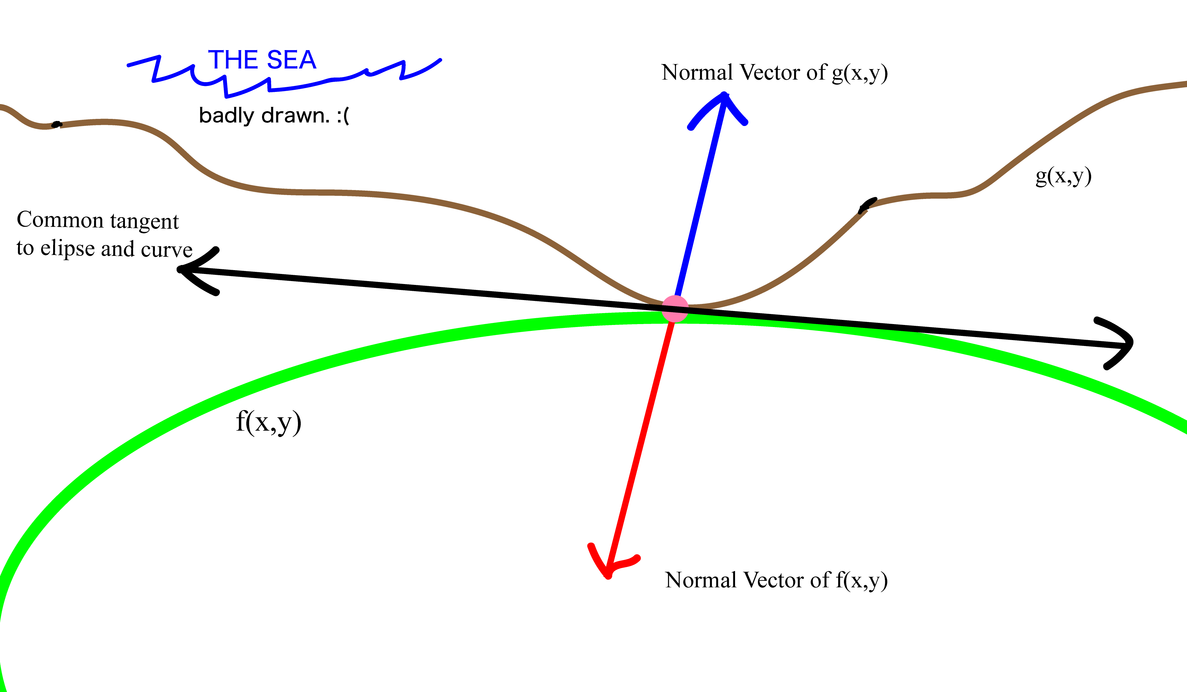
A lot of interesting stuff happens here at the interection point. First, you can easily verify that both the curves have a common tangent equations. Nice. Next, the point has two normals acting on it, in the opposite directions. This is what we care about.
Normals.Let’s focus on normals. As we know the normal is given by the gradient of the curve, (since the gradient of a function is perpendicular to the contour lines)
and,
So, we never know whether these normal are balanced. It depends on the curve and elipse equations. Thus we introduce a scalar, non-zero constant, $\lambda$ (to balance the point of interection, where the maxima or minima lies).
This constant is called the Lagrange multiplier.
We continue solving this equation,
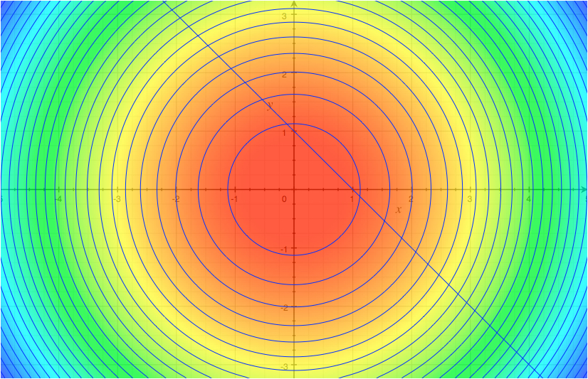
Note, setting $\lambda = 0$ is a solution if $f(x,y)$ is at the level (horizontal) regardless of $g(x,y)$.
Let us define another function $\mathscr{L}(x,y,\lambda) \equiv f(x,y) + \lambda g(x,y)$ to include all the conditions into one equation and solve for $\nabla_{x,y,\lambda}\mathscr{L}(x,y,\lambda) = 0.$ [ this function is also called the Lagrangian Function, also note that $\lambda$ can be positive or negative ]
As there are three unknowns, $x,y$ and $\lambda$, would need to solve three equations.
The constraint condition, $\nabla_{x,y} f = \lambda \nabla_{x,y} g $ is found by setting $\nabla_x \mathscr{L} = 0$ and further, the condition $\nabla_{\lambda} \mathscr{L}(x,y,\lambda) = 0$ leads to $g(x,y) = 0$.
An example will make this much more clear.
Answer.
I hope this example made the concept much clear! Let’s move forward and discuss Lagrangian Multipliers with some physics!
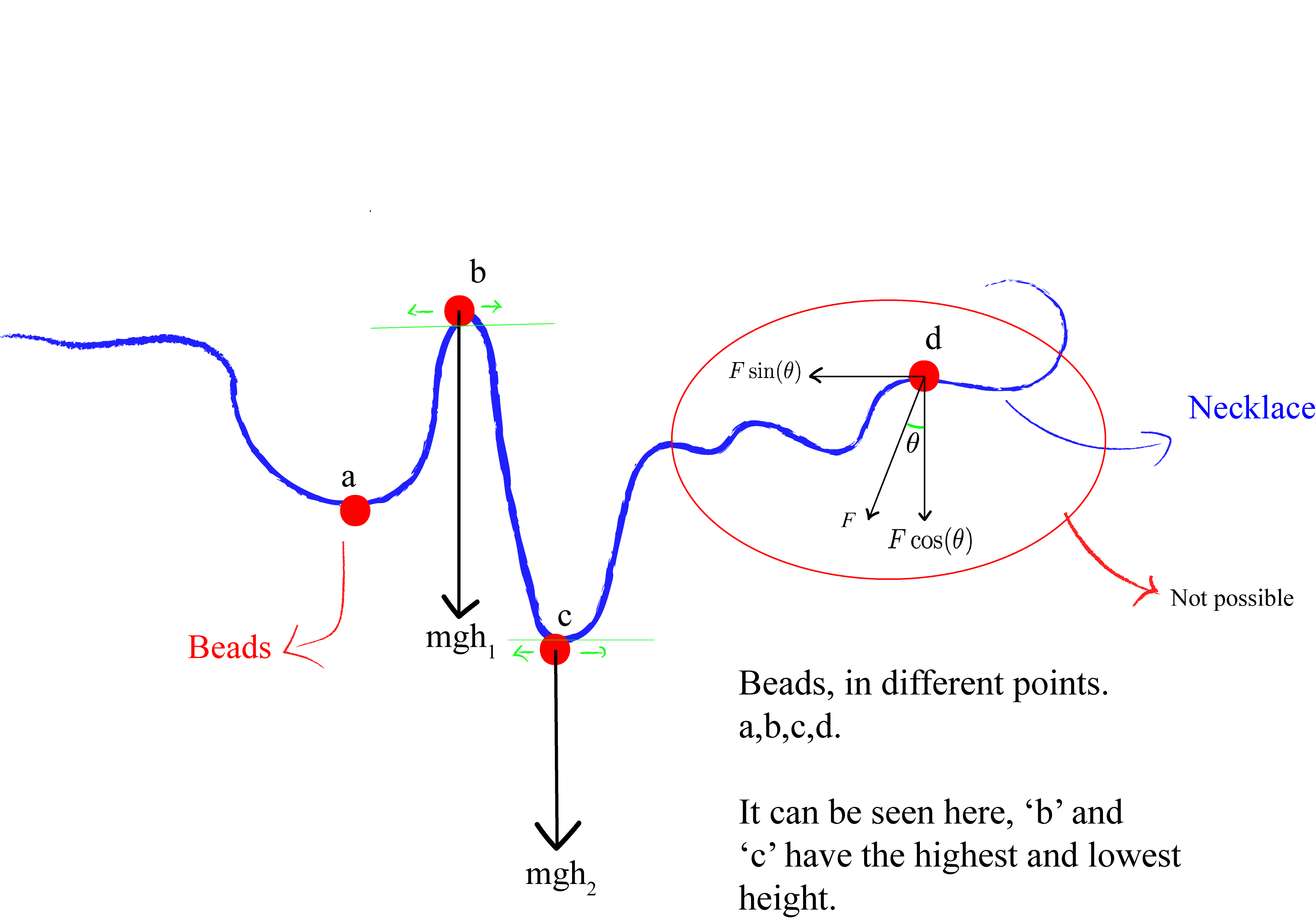
The Necklace
This section is more on the the physical approach in understanding why we don’t consider the tangent but the normal.
The points $a,b,c,d$ are the points where the necklace is perpendicular to the downward force and only at these points the normal reaction ( $F$ ) is balanced by the gravitional potential $\phi = mgh$.
As it’s balanced ( if not the necklace won’t be parallel to the surface) we get,
Let’s forget about the other points and only consider $d$ and say this is where the maximum occurs. Then it can be seen that $\nabla F$, the gradient of $F$ must be perpedicular to the necklace at $d$. If any component of $\nabla F$ were parallel we could move away from $d$ and arive at another point which would be the maxima contrary to our claim that $d$ is the maxima. Thus,
Another way is looking closely at point $d$ for which a force $F$ acts at angle $\theta$ and we can find the components of this force as $F\cos \theta $ and $F\sin \theta $. Now as it’s a stationary point,
…..which again proves that $\nabla F \perp$ Necklace.
Few Words
I hope this post has been a bit helpful in visually understandng what Lagrangian Multipliers through geometric explorations. As always recap,
References include my father’s lecture notes on numerical methods and FEM at NITC (riverbed), Wikipedia, math.stackexchange, Pattern Recognition and Machine Learning, Bishop and MIT OWC Multivariable Calculus. (necklace intuition)
All images are mine and are licensed under CC-BY-4.0. Softwares used include MATLAB, OSX Grapher and Adobe Illustrator.
I hope you had as much fun reading than I had writing this up!
Wish you all a happy near year 2018!
Ankit.